Co-wrote these with Sandra Romero Pinto
Notes summarizing Nonlinear Dynamics and Chaos
In general, we’re interested in functions $x : \mathbb{R^n}\to\mathbb{R^m}$ satisfying some differential equation $x’(t)=f(x(t))$, so that their local linearizations at a point are linear maps also of $\mathbb{R^n}\to\mathbb{R^m}$. Note that this is a first order differential equation, but higher order ones can be reformulated as first order by considering $x, x’, x”…$ as a vector of variables.
When $f$ is a linear map, the solution takes the form $e^{ft}$ and everything is nice, because linear algebra provides powerful tools that are applicable in this case. But when $f$ is not a linear map, things can be hard. Calculus provides a powerful tool for handling non-linear systems, namely that the first order approximation of a non-linear system is linear. Sometimes the linear approximations tell you everything important about the non-linear system (see the Hartman-Grobman theorem). Often, however, even this isn’t enough. For the most part, this book is interested in the second case.
A general theme of the book is to think geometrically and topologically, but looking at the kinds of solutions available. Of particular interest are fixed points, which are points $x^*$ where $f(x’)=0$, called as such because if you start at such a point, you stay at it. In the jargon of ODEs: fixed points are the equilibrium solutions (constant solutions).
There’s an intuitive notion of stability of fied points, namely whether arbitrarily small pertubations of a fixed point result in a return to the fixed point (stable) or not (unstable). See more on this below.
Fixed points are a sort of topological feature of an ODE, in the sense that we can qualitatively characterize a solution by asking about the number and stability of its fixed points, rather than finding the exact value of $x$ at all $t$.
This leads naturally to the notion of a bifurcation, where you have an ODE parametrized by some parameter $p \in \mathbb{R}$ and as you vary $p$, you find that at some point the number or stability of the fixed points changes. This is a bifurcation.
Another theme of this book is that graphical analysis can be used to determine fixed points, and more generally make our lives a lot easier.
Linear Stability Analysis
We can be clever about analyzing stability by forming a new ODE in terms of a perturbation around a fixed point. That is, for a fixed point $x_0$, and in the 1D case:
$$ \eta(t) := x(t)-x_0 $$
Then it follows that:
$$ \dot{\eta} = \dot{x} = f(x) = f(\eta+x_0) = f(x_0) + \eta f’(x_0)+O(\eta^2) = \eta f’(x_0)+O(\eta^2) \approx \eta f’(x_0) $$
This final approximation is true for $f’(x^*)\neq 0$ in the limit of small $\eta$. Solving this ODE ($\dot{\eta}=\eta f’(x_0)$) shows that for $f’(x_0)>0$, the perturbation grows, and for $f’(x_0)<0$ is shrinks, returning the trajectory back to the fixed point. For $f’(x_0)=0$ we’re back to square one.
This generalizes to the n-dimensional case (see these ODE notes), where $f’$ becomes the Jacobian. Then, the case of all eigenvalues with negative real part gives stability, all positive real part gives instability. More generally if all eigenvalues have a real part, this is known as a hyperbolic fixed point. The cases where at least one eigenvalue has real part $0$ are the difficult ones, as the linearization around a fixed point doesn’t always reflect the true phase portrait of the non-linear system
Definitions to describe stability of fixed points (linear/nonlinear)
Considering $\textbf{x}^*$ the fixed point of a dynamical system:
- $\textbf{x}^*$ is an attracting point if $x(t) \to \textbf{x}^*,\text{as}, t \to \infty $ (trajectories starting near it eventually converge to $\textbf{x}^*$) . It can be called globally attracting if it attracts all trajectories (but sometimes it has a certain basin of attraciton. Focuses on the condition of $t \to \infty$
- $\textbf{x}^*$ is a Lyapunov stable: if trajectories starting sufficiently close to $\textbf{x}^*$,remain close to it at all times.
A given $\textbf{x}^*$ can be both attracting and Lyapunov stable, or only either.
- $\textbf{x}^*$ can be attracting but not Lyapunov stable: if trajectories actually diverge from the fixed point to then converge on it as $t \to \infty $ (no particular name for this)
- If it’s only Lyapunov stable then $\textbf{x}^*$ is neutrally stable: trajectories remain near it but never actually converge on it.
- If it’s both, $\textbf{x}^*$ is asymptotically stable
- if it’s neither, $\textbf{x}^*$ is unstable
1D ODEs
For $x : \mathbb{R}\to\mathbb{R}$, the kinds of solutions are limited (all solutions either approach a fixed point or diverge to $\pm\infty$, as are the kinds of birfurcations.
The following is a list of the kinds of birfurcations in 1D. For each kind, I list the normal forms. These are simple ODEs which provide an example of the kind of bifurcation, but note that not all bifurcations are of the normal form. For example, $\dot{x}=-x + \beta\tanh x$ has a saddle node bifurcation. However, to a first order approximation (i.e. locally) the normal form is equivalent to any other bifurcation of that class. (Actually Strogatz alludes to something else, see this page, namely a topological equivalence of the normal form to other members of its class. I think the mathematical content of this is probably a bit sophisticated, but informally I think it just means that the qualitative behavior of fixed points and their stability is the same.)
Normal forms are therefore the 1st order approximation to all these canonical bifurcations. Here are the 1D normal forms:
- saddle-node bifurcations: at which the number of fixed point changes
- normal forms: $x^2 - r$ and $x^2 + r$
- normal forms: $x^2 - r$ and $x^2 + r$
- transcritical bifurcations: at which the fixed points change their stability
- normal forms: $ rx - x^2$
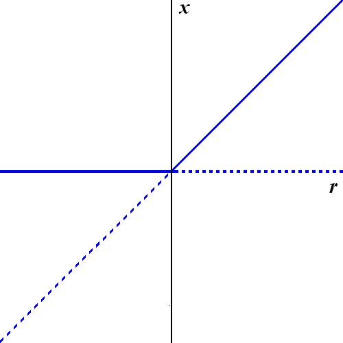
- normal forms: $ rx - x^2$
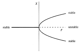
- pitchfork bifurcations: number of fixed point changes but also the stability changes (…). The core feature is that the system has symmetry (it behaves the same if $x\mapsto -x$ ). Can be sub-or supercritical depending on the stability of the remaining fixed points after the bifurcation (the names are counter-intuitive for the stability of the remaining fixed points)
- supercritical normal form: $ rx - x^3$
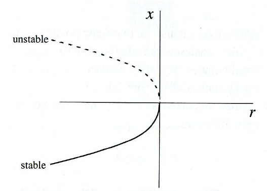
- subcritical normal form: $ rx + x^3$
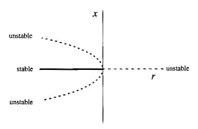
- subcritical with hysteresis: $rx + x^3 - x^5$
- supercritical normal form: $ rx - x^3$
As an example of a complicated ODE which takes a well-known normal form in the 1st order, consider:
$$ \dot{x} = r\ln x + x -1 $$
For $u := x -1$, $\dot{u} = r\ln(1+u)+u = r[u-\frac{1}{2}u^2 + O(u^3)] + u = (r+1)u - \frac{1}{2}ru^2 + O(u^3)$. Up to rescaling, this is the normal for for a supercritical pitchfork bifurcation.
Usefulness of graphs
Stability of a fixed point can be determined by just looking at the vector field of the system: in a 1D system, this is given by an $\dot{x}$ against $x$ graph.
Points crossing the x-axes are the fixed points and the stability can just be determined by looking at the sign of $\dot{x}$ around that fixed point (basically checking whether x would approach or diverge from that fixed point given the sign of the derivative $\cdot{x}$). - This is very similar to doing perturbation analysis and linearization around a fixed point to determine its stability, but in a graphical - much nicer to look at - way .
2D ODEs
Some common kinds of fixed points include:
Limit cycles
They are closed & isolated trajectories, meaning that the trajectories neighboring it are not closed but are spirals toward (stable limit cycle) or away (unstable limit cycle) to /from it. Sometimes they can be half-stable (toward or away from it inside or outside of the closed trajectory) . They are inherent of nonlinear systems, as closed orbits in linear systems can’t be isolated by the definition above, and in contrast form families of closed orbits whose amplitude is scaled by a constant (determined by the initial conditions and preserved, there can never be spirals in linear systems).
Limit cyles can’t exist if a Lyapunov function exists for the system. Intuitively, this is an energy-like function that decreases along trajectories. More formally: it’s a continuously differentiable real-valued function $V(\textbf{x})$ that : 1) is positive definite : $V(\textbf{x})>0 ~ \forall \textbf{x} \neq \textbf{x}^* , V(\textbf{x}^*)=0$ , 2) for which all trajectories go downhill in the V function towards $\textbf{x}^*$ : $\dot{V}<0 ~ \forall \textbf{x} \neq \textbf{x}^*$.
Focusing on property 2) this would make the fixed point to be globally stable (all trajectories move towards is) and would make it impossible to have a closed trajectory (i.e. limit cycle) as this would imply that $\dot{V} =0$.
Other ways of ruling out limit cycles are by determining whether the system is gradient system (very similar to figuring out whether a Lyapunov function exists), and Dulac’s criterion. The Poincaré-Bendixson theorem is used to determine whether a closed orbit exists in a system.
Bifurcations
All the 1D cases still apply, but there are now some more cases too. In 1D, eigenvalues lie on the real line, but in 2 or more dimensions, they can be complex. In particular, for 2D, the eigenvalues are the solution of a quadratic equation with real coefficients (see linear algebra notes), so if $4ac$ is non-negative, they are both real, and if $4ac$ is negative, they are both complex conjugates (because $\sqrt{4ac}$ is purely imaginary, it’s negative is its conjugate, and then the other terms of the quadratic formula shift and scale along the real axis).
So now we have a new case, where the change of stability occurs when both eigenvalues cross the imaginary axis at once. These are Hopf bifurcations.
Of these, we have supercriticial and subcritical Hopf bifurcations.
Supercritical Hopf bifurcations
Conceptually, the former are the onset or stopping of a vibration. Graphically, these are changes from stable spirals to unstable ones which head towards a limit cycle.
For example:
$$ \dot{r} = \mu r - r^3$$
$$ \dot{\theta} = \omega + br^2 $$
https://www.google.comgitFirst note that the top https://www.google.comgitequation is just a 1D supercritical pichtfork bifurcation. But the change to polar means that $\theta$ lives on S1 (the circle), so 2D really is adding something here, because stability for $r$ now means oscillation.
We can see that for $\mu>0$ we get a limit cycle when $\sqrt{\mu}=r$ . For $\mu \leq 0$, we have a spiral at the origin. So when $\mu$ becomes positive, the origin becomes unstable and small perturbations from it result in an escape towards the $\sqrt{\mu}=r$ limit cycle.
Subcritical Hopf bifurcation
For example,
$$ \dot{r} = \mu r + r^3 - r^5$$
$$ \dot{\theta} = \omega + br^2 $$
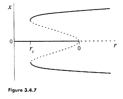
As above, but now the first equation is a subcritical pitckfork with hysteresis, in $r$. The cubic term is now positive and thus destabilizing. Unlike the 1D example, with the following diagram, $r$ is now always non-negative, so only consider the top half of the diagram:
Note: don’t get confused by the label names: the parameter is now called $\mu$, not $r$, and the variable is now called $r$, not $x$.
Now what follows, which you can see from the diagram, is that as $\mu$ increases towards $0$, the unstable branch, which now represents an unstable cycle, constricts around the origin, and when it engulfs it, renders the origin unstable too. Then, perturbations from the origin result in a jump to the larger stable cycle, and there’s hysteresis, because decreasing $\mu$ below $0$ doesn’t return the system to the initial trajectory. Saddle- node bifurcation of cycles
Similarly to the 1D system in which the number of fixed point changes for a saddle-node bifurcation, in a 2D system it is the number of limit cycles that changes. Usually thought as two limit cycles colliding and then disappearing.
Prototypical system (the same analyzed for the subcritical Hopf bifurcation but $$\mu <0$$ always
$$ \dot{r} = \mu r + r^3 -r^5$$
$$\dot{\theta} = \omega + b r ^2$$
In this system, the parameter has a critical value $$\mu_c$$ at which the system goes from having a stable spiral at origin $$\mu<\mu_c$$ , to having a half stable spirla at $$\mu=\mu_c$$ , to having a stable and an unstable limit cycles for $$\mu>\mu_c$$ . Very much analogue to the 1D system that ends up having a stable and unstable branch.
Coupled systems
Of the form: $$\dot{\theta_1} = f_1(\theta_1, \theta_2)\ \dot{\theta_2} = f_2(\theta_1, \theta_2)$$ , with $$f_1, f_2$$: being periodic in both arguments
a simple one would be : $$\dot{\theta_1} = \omega_1+ K_1 \sin (\theta_2-\theta_1)\ \dot{\theta_2} = \omega_2+ K_2 \sin (\theta_2-\theta_1)$$
the coupling constants ($$K_1, K_2$$) determine the strength and presence of coupling. A way to represent the system is through a torus in which there are two axes of rotation, each with a coordinate ($$\theta_1, \theta_2$$) that represent the phase of each oscillator. But an easier way is to make use of a square representation with periodic boundary conditions at its edges.
An uncoupled oscillator occurs when $$K_1 = K_2 = 0$$ and thus the each oscillator oscillates at its natural frequency ($$\omega_1, \omega_2$$). In a square representation, this system results in straight lines and the slope is the ratio of the natural frequencies: $$\frac{d\theta_1}{d\theta_2} = \frac{\omega_1}{\omega_2}$$. If the ratio is rational, then the system is periodic and the trajectories form closed orbits; but if the ratio is irrational the system is quasiperiodic, each trajectory never closes on itself ,and ends in a point near to the starting point.
A coupled oscillator occurs when $$K_1 , K_2 > 0$$ . In a system like the one above, we study its dynamics by looking at the phase difference, and we end up with a 1D system: $$\phi = \theta_1- \theta_2\ \dot{\phi} = \dot{\theta_1}- \dot{\theta_2} = \omega_1 -\omega_2 -(K_1+K_2) \sin \phi \ $$
This system goes through a saddle node bifurcation at $$|\omega_1 -\omega_2| = (K_1+K_2) $$.
When the system has 2 fixed points $$(K_1+K_2) >|\omega_1 -\omega_2| $$, all trajectories approach the stable point which here is the point at which the phase difference $$\phi$$ doesn’t change $$\dot{\phi} =0$$, and the system oscillates at a constant phase difference (i.e. oscillators are phase locked). In this solution, the system is periodic and both oscillators run at a constant compromise frequency : a weighted average of their natural frequencies (weighted by the coupling constants)
The bifurcation is intuitive: if the the two natural frequencies become too different ($$|\omega_1 -\omega_2|>(K_1+K_2) $$) then the coupling strengths can’t keep the system phase locked and the system behaves like the uncoupled system above.
Poincare maps
These are a nice way to figure out whether there are closed orbits in the system, and whether these orbits are stable or unstable. It’s a way of reformulating a problem about orbits in a system into a problem of fixed points of a iterated map.
Graphically, one can imagine drawing a section or plane S of (n-1) dimensions, where n is the system’s dimension. The trajectories traverse these plane but don’t run parallel to it.
The Poincare map P is a mapping from the plane S to itself: it looks at consecutive intersections of the trajectories of the system with S: $$\textbf{x}{k+1} = P(\textbf{x}{k})$$
If the mapping function $$P(x)$$ has a fixed point for x : $$\textbf{x}^* = P(\textbf{x}^*)$$ , then the system is intersecting itself in $$\textbf{x}^* $$ and thus it would have to be a closed orbit in the original system of interest $$ \dot{\textbf{x}} = f(\textbf{x}) $$. One can then look at the behavior of the mapping P at nearby points to $$\textbf{x}^* $$ to check for stability conditions.
Index Theory
(The book describes this in 2D; it presumably generalizes, although I don’t know how.)
The index or winding number of a curve (but not necessarily a trajectory) in the phase plane is the number of times the vector field rotates counterclockwise around if you integrate its angle along the path (it can be signed and so it’s worth talking about the net number of turns along the curve)
Here’s the relevant property of the winding number: it is an invariant under homotopies, i.e. transformations which don’t move the curve across fixed points. This is because it is always an integer ($k \pi$), so can’t change continuously, other than to be constant (if an integer value function is continuous it can only be constant else it jumps) . Note, at a fixed point, the vector field points in no direction, so winding number isn’t defined on curves through fixed points.
Secondly: the winding number is equal to the sum of the indeces of the isolated fixed points it surrounds. As a special case: if there are no fixed points, the winding number is $0$. This is proven basically by contracting the curve very tightly around the fixed points and cancelling out the paths in between.
(Note that this is basically the same mathematics as the residue theorem in complex analysis, although I couldn’t exactly spell out the details of the analogy.)
The index of a saddle point is $-1$ and of a spiral or center: $+1$.
Worked examples
Example: $\dot{x} = -x + \beta\tanh x$ : model of the phase transition of a mean-field approximation to the 2D Ising model (see statistical mechanics notes ).
Example: simple model of a laser:
$$ \dot{n} = (GN_0-k)n - (\alpha G)n^2$$
where $n$ is the number of photons. This is, up to a scaling, in the normal form of a transcritical bifurcation, and this bifurcation at $k/G$ represents where lasing happens.
Example: The pendulum: $\frac{d^2\theta}{dt^2}+\frac{g}{L}\sin\theta$. It’s traditional to solve by a local linearization. Instead we’ll do the typical thing of this book, and characterize the fixed points. First, we non-dimensionalize (see these notes on dimensions), to obtain $\ddot{\theta}=-\sin\theta$ and from that, the first order system $\dot{\theta}=v, \dot{v}=-\sin\theta$. The fixed points, modulo periodicity, are $(0,0)$ and $(k\theta,0)$. There are various ways to show that the first is a center (through the reversibility or conservativity of the system), but rigorous proofs require some doing. However, the second is, up to linearization, a saddle, since the Jacobian is:
$$ \begin{bmatrix}
\frac{dv}{d\theta} & \frac{dv}{dv}
\frac{-d\sin\theta}{d\theta} & \frac{-d\sin\theta}{d\theta}
\end{bmatrix}|_{(k\pi,0)} = \begin{bmatrix}
0 & 1
1 & 0
\end{bmatrix}$$
which has eigenvalues as solutions of $\lambda^2-1=0$, namely $-1$ and $1$. Thus it’s a hyperbolic fixed point, and so this goes for the original non-linear system too.
Example 5.1.2 Intuition on drawing trajectories wrt eigenvalues and fixed points
Conservative Systems
These are ODEs for which there’s a conserved quantity (but non-constant on open sets to avoid $E(x)=0$ witnessing conservativity trivially for all ODEs), the obvious example being Hamiltonian classical mechanics. An immediate consequence is that there can’t be an attracting fixed point, since then the conserved quantity would be constant on the open set leading to the fixed point.
Conservative systems also make nonlinear centers to become more robust to the linearization approximation around fixed points (in nonconservative systems centers are very delicate and small perturbations can destroy them and make them become spirals) . In conservative systems, because energy (or any other quantity) is preserved within a given trajectory, then they can be thought of ‘contours’ of a constant Energy level c: $E(x)=c $. If a fixed point $\textbf{x}^*$ is a minima or maxima of $E(x)$, and there are no other fixed points in a close neighborhood (i.e.$\textbf{x}^*$ is isolated) then trajectories close to it need to be closed (think about energy ‘wells’ in 2D), making $\textbf{x}^*$ a center. (Theorem 6.5.1 : Nonlinear centers for conservative systems)
Chaos
The original and typical example is the Lorenz equations. These are a 3D ODE whose long term behavior is not convergence to a fixed point or limit cycle, but is confined to a bounded region. Note that this would violate Poincaré-Bendixson in 2D. The surprising conclusion is that the long-term behavior converges to a strange attractor, which is a set of measure $0$ not unlike the Cantor set.
Important theorems
None of these are particularly easy to use without being quite clever first. For example, Poincaré-Bendixson requires you to find a confining (or “trapping”) region, to ensure the trajectory is inside a closed region, and there isn’t a generic way to do this.
Poincaré-Bendixson theorem: roughly, if you have a trajectory that you know to be confined to a closed region of the phase plane in 2D, and the region contains no fixed points, then it’s either a closed orbit or converges to one. So there’s no chaos in the phase plane (chaos being the alternative to converging to a closed orbit).
Hartman-Grobman: there’s a notion of topological equivalence of phase portraits which I won’t try to define, but is intuitive, namely: smooth invertible deformation mapping trajectories onto trajectories, fixed points onto fixed points, etc, that allows the sense of time in the trajectories between the mappings to be preserved. This theorem states that the local linearization of an equation around a hyperbolic fixed (has to be hyperbolic*) point is topologically equivalent to the original equation.
Glossary
- hysteresis: the phenomenon where you vary a parameter, by say increasing it, waiting for the system to stabilize, and then decreasing it back to where you started, and finding that the system does not return to the original behavior. For example, looking at the bifurcation diagram for $rx + x^3 - x^5$, we can see that if you increase $r$ past $0$, and stability is lost, there is a jump to a new branch, and decreasing $r$ below $0$ again with not restore you to the old branch, until you get below $r_s$.
- ghost: a saddle birfucation like $\dot{x} = r +x^2$, for example, once gone (i.e. for $r > 0$), involves a parabola almost touching the x-axis, so we can calculate the time to pass through as $\int{-\infty}^{\infty}dt = \int{-\infty}^{\infty}\frac{dt}{dx}dx = \int_{-\infty}^{\infty}\frac{1}{r+x^2}dx = \frac{\pi}{\sqrt{r}} $ which gives a characteristic $r^{-\frac{1}{2}}$ scaling law.
- iterated map: a discrete version of an ODE
- That famous bifurfaction diagram:

- OK, here’s what this is a diagram of. We have an iterated map, e.g. $x_{n+1} = rx_n(1-x_n)$. $r$ is being varied on the x-axis. The values which $x_n$ (asymptotically) inhabits are on the y-axis. As the diagram shows, we have bifurcation values at which the periodicity of the system doubles, but what’s most interesting is that we get to a point where the exponential increase from the doubling hits a crescendo and leads to a vertical whitespace column